As usual, our starting point is a random experiment, modeled by a probability space $(\mathrm{\Omega },\mathcal{F},P)$. So to review, $\mathrm{\Omega }$ is the set of outcomes, $\mathcal{F}$ the collection of events, and $\mathbb{P}$ the probability measure on the sample space $(\mathrm{\Omega },\mathcal{F})$. Suppose that $X$ is a real-valued random variable for the experiment. Recall that the mean of $X$ is a measure of the center of the distribution of $X$. Furthermore, the variance of $X$ is the second moment of $X$ about the mean, and measures the spread of the distribution of $X$ about the mean. The third and fourth moments of $X$ about the mean also measure interesting (but more subtle) features of the distribution. The third moment measures skewness, the lack of symmetry, while the fourth moment measures kurtosis, roughly a measure of the fatness in the tails. The actual numerical measures of these characteristics are standardized to eliminate the physical units, by dividing by an appropriate power of the standard deviation. As usual, we assume that all expected values given below exist, and we will let $\mu =\mathbb{E}(X)$ and ${\sigma }^2=\text{var}(X)$. We assume that $\sigma >0$, so that the random variable is really random.

Basic Theory

Skewness

In the unimodal case, if the distribution is positively skewed then the probability density function has a long tail to the right, and if the distribution is negatively skewed then the probability density function has a long tail to the left. A symmetric distribution is unskewed.

The converse is not true—a non-symmetric distribution can have skewness 0. Examples are given in [30] and [31].

Since skewness is defined in terms of an odd power of the standard score, it's invariant under a linear transformation with positve slope (a location-scale transformation of the distribution). On the other hand, if the slope is negative, skewness changes sign.

Recall that location-scale transformations often arise when physical units are changed, such as inches to centimeters, or degrees Fahrenheit to degrees Celsius.

Kurtosis

Kurtosis comes from the Greek word for bulging. Kurtosis is always positive, since we have assumed that $\sigma >0$ (the random variable really is random), and therefore $\mathbb{P}(X\ne \mu )>0$. In the unimodal case, the probability density function of a distribution with large kurtosis has fatter tails, compared with the probability density function of a distribution with smaller kurtosis.

Since kurtosis is defined in terms of an even power of the standard score, it's invariant under linear transformations.

We will show in that the kurtosis of the standard normal distribution is 3. Using the standard normal distribution as a benchmark, the excess kurtosis of a random variable $X$ is defined to be $\text{kurt}(X)-3$. Some authors use the term kurtosis to mean what we have defined as excess kurtosis.

Computational Exercises

As always, be sure to try the exercises yourself before expanding the details.

Indicator Variables

Recall that an indicator random variable is one that just takes the values 0 and 1. Indicator variables are the building blocks of many counting random variables. The corresponding distribution is known as the Bernoulli distribution, named for Jacob Bernoulli.

Dice

Recall that a fair die is one in which the faces are equally likely. In addition to fair dice, there are various types of crooked dice. Here are three:

• An ace-six flat die is a six-sided die in which faces 1 and 6 have probability $\frac{1}{4}$ each while faces 2, 3, 4, and 5 have probability $\frac{1}{8}$ each.
• A two-five flat die is a six-sided die in which faces 2 and 5 have probability $\frac{1}{4}$ each while faces 1, 3, 4, and 6 have probability $\frac{1}{8}$ each.
• A three-four flat die is a six-sided die in which faces 3 and 4 have probability $\frac{1}{4}$ each while faces 1, 2, 5, and 6 have probability $\frac{1}{8}$ each.

A flat die, as the name suggests, is a die that is not a cube, but rather is shorter in one of the three directions. The particular probabilities that we use ($\frac{1}{4}$ and $\frac{1}{8}$) are fictitious, but the essential property of a flat die is that the opposite faces on the shorter axis have slightly larger probabilities that the other four faces. Flat dice are sometimes used by gamblers to cheat.

All four die distributions above have the same mean $\frac{7}{2}$ and are symmetric (and hence have skewness 0), but differ in variance and kurtosis.

Uniform Distributions

Recall that the continuous uniform distribution on a bounded interval corresponds to selecting a point at random from the interval. Continuous uniform distributions arise in geometric probability and a variety of other applied problems.

The Exponential Distribution

Recall that the exponential distribution is a continuous distribution on $[0,\mathrm{\infty })$with probability density function $f$ given by $$f(t)=r{e}^{-rt},t\in [0,\mathrm{\infty })$$ where $r\in (0,\mathrm{\infty })$ is the with rate parameter. This distribution is widely used to model failure times and other arrival times, particulalry in the context of the Poisson model.

Note that the skewness and kurtosis do not depend on the rate parameter $r$. That's because $1/r$ is a scale parameter for the exponential distribution

Pareto Distribution

Recall that the Pareto distribution is a continuous distribution on $[1,\mathrm{\infty })$ with probability density function $f$ given by $$f(x)=\frac{a}{x^{a+1}},x\in [1,\mathrm{\infty })$$ where $a\in (0,\mathrm{\infty })$ is a parameter. The Pareto distribution, named for Vilfredo Pareto, is a heavy-tailed distribution that is widely used to model financial variables such as income.

The Normal Distribution

Recall that the standard normal distribution is a continuous distribution on $\mathbb{R}$ with probability density function $\varphi$ given by $$\varphi (z)=\frac{1}{\sqrt{2\pi }}{e}^{-\frac{1}{2}{z}^2},z\in \mathbb{R}$$ Normal distributions are widely used to model physical measurements subject to small, random errors.

More generally, for $\mu \in \mathbb{R}$ and $\sigma \in (0,\mathrm{\infty })$, recall that the normal distribution with mean $\mu$ and standard deviation $\sigma$ is a continuous distribution on $\mathbb{R}$ with probability density function $f$ given by $$f(x)=\frac{1}{\sqrt{2\pi }\sigma }\exp [-\frac{1}{2}{\left(\frac{x-\mu }{\sigma }\right)}^2],x\in \mathbb{R}$$ However, we also know that $\mu$ and $\sigma$ are location and scale parameters, respectively. That is, if $Z$ has the standard normal distribution then $X=\mu +\sigma Z$ has the normal distribution with mean $\mu$ and standard deviation $\sigma$.

The Beta Distribution

The distributions in this subsection belong to the family of beta distributions, which are continuous distributions on $[0,1]$ widely used to model random proportions and probabilities.

The particular beta distribution in the last exercise is also known as the (standard) arcsine distribution. It governs the last time that the Brownian motion process hits 0 during the time interval $[0,1]$.

Counterexamples

The following exercise gives a simple example of a discrete distribution that is not symmetric but has skewness 0.

The following exercise gives a more complicated continuous distribution that is not symmetric but has skewness 0. It is one of a collection of distributions constructed by Erik Meijer.

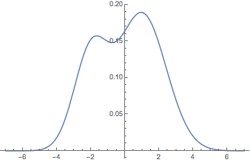
Suppose that $U$, $V$, and $I$ are independent random variables, and that $U$ is normally distributed with mean $\mu =-2$ and variance ${\sigma }^2=1$, $V$ is normally distributed with mean $\nu =1$ and variance ${\tau }^2=2$, and $I$ is an indicator variable with $\mathbb{P}(I=1)=p=\frac{1}{3}$. Let $X=IU+(1-I)V$. Find each of the following and then show that the distribution of $X$ is not symmetric.

1. $\mathbb{E}(X)$
2. $\text{var}(X)$
3. $\text{skew}(X)$
4. $\text{kurt}(X)$

Details:

The distribution of $X$ is a mixture of normal distributions. The PDF is $f=pg+(1-p)h$ where $g$ is the normal PDF of $U$ and $h$ is the normal PDF of $V$. However, it's best to work with the random variables. For $n\in {\mathbb{N}}_{+}$, note that $I^n=I$ and $(1-I{)}^n=1-I$ and note also that the random variable $I(1-I)$ just takes the value 0. It follows that $$X^n=I{U}^n+(1-I)V^n,n\in {\mathbb{N}}_{+}$$ So now, using standard results for the normal distribution,

1. $\mathbb{E}(X)=p\mu +(1-p)\nu =0$.
2. $\text{var}(X)=\mathbb{E}(X^2)=p({\sigma }^2+{\mu }^2)+(1-p)({\tau }^2+{\nu }^2)=\frac{11}{3}$
3. $\mathbb{E}(X^3)=p(3\mu {\sigma }^2+{\mu }^3)+(1-p)(3\nu {\tau }^2+{\nu }^3)=0$ so $\text{skew}(X)=0$
4. $\mathbb{E}(X^4)=p(3{\sigma }^4+6{\sigma }^2{\mu }^2+{\mu }^4)+(1-p)(3{\tau }^4+6{\tau }^2{\nu }^2+{\nu }^4)=31$ so $\text{kurt}(X)=\frac{279}{121}\approx 2.306$

The graph of the PDF $f$ of $X$ is given below. Note that $f$ is not symmetric about 0. (Again, the mean is the only possible point of symmetry.)